Setting up a model
We are going to implement a simple linear decay equation:
Where \(T\) is the temperature in Kelvin, \(a>0\) is the linear constant and \(F\) the forcing parameter.
To set up the model, some straight-forward steps are necessary. First,
import the numericalmodel module:
import numericalmodel
Creating a model
First initialize an object of NumericalModel:
model = numericalmodel.numericalmodel.NumericalModel()
We may tell the model to start from time \(0\):
model.initial_time = 0
Defining variables, parameters and forcing
The StateVariable, Parameter, and ForcingValue classes all
derive from InterfaceValue, which is a convenient class for time/value
management. It also provides interpolation (InterfaceValue.__call__). An
InterfaceValue has a (sensibly unique) id for it to be
referencable in a SetOfInterfaceValues.
For convenience, let’s import everything from the interfaces submodule:
from numericalmodel.interfaces import *
Let’s define our state variable. For the simple case of the linear decay equation, our only state variable is the temperature \(T\):
temperature = StateVariable( id = "T", name = "temperature", unit = "K" )
Providing a name and a unit documents your model on the fly.
Tip
All classes in numericalmodel are subclasses of
ReprObject. This makes them have a proper __repr__ method to
provide an as-exact-as-possible representation. So at any time you might do a
print(repr(temperature)) or just temperature<ENTER> in an
interactive python session to see a representation of this object:
numericalmodel.interfaces.StateVariable(
        unit = 'K',
        bounds = [-inf, inf],
        name = 'temperature',
        times = array([], dtype=float64),
        time_function = numericalmodel.utils.utcnow,
        id = 'T',
        values = array([], dtype=float64),
        interpolation = 'zero'
        )
The others - \(a\) and \(F\) - are created similarly:
parameter = Parameter( id = "a", name = "linear parameter", unit = "1/s" )
forcing = ForcingValue( id = "F", name = "forcing parameter", unit = "K/s" )
Now we add them to the model:
model.variables  = SetOfStateVariables( [ temperature ] )
model.parameters = SetOfParameters(     [ parameter ]   )
model.forcing    = SetOfForcingValues(  [ forcing ]     )
Note
When an InterfaceValue‘s value is set, a corresponding
time is determined to record it. The default is to use the return value of
the InterfaceValue.time_function, which in turn defaults to the
current utc timestamp. When the model was told to use temperature,
parameter and forcing, it automatically set the
InterfaceValue.time_function to its internal model_time. That’s
why it makes sense to define initial values after adding the
InterfaceValue s to the model.
Now that we have defined our model and added the variables, parameters and forcing, we may set initial values:
temperature.value = 20 + 273.15
parameter.value   = 0.1
forcing.value     = 28
Tip
We could also have made use of SetOfInterfaceValues‘ handy
indexing features and have said:
model.variables["T"].value  = 20 + 273.15
model.parameters["a"].value = 0.1
model.forcing["F"].value    = 28
Tip
A lot of objects in numericalmodel also have a sensible
__str__ method, which enables them to print a summary of themselves. For
example, if we do a print(model):
###
### "numerical model"
### - a numerical model -
###  version 0.0.1
###

by:
anonymous

a numerical model
--------------------------------------------------------------
This is a numerical model.


##################
### Model data ###
##################

initial time: 0

#################
### Variables ###
#################

 "temperature"
--- T [K] ---
currently: 293.15 [K]
bounds: [-inf, inf]
interpolation: zero
1 total recorded values

##################
### Parameters ###
##################

 "linear parameter"
--- a [1/s] ---
currently: 0.1 [1/s]
bounds: [-inf, inf]
interpolation: linear
1 total recorded values

###############
### Forcing ###
###############

 "forcing parameter"
--- F [K/s] ---
currently: 28.0 [K/s]
bounds: [-inf, inf]
interpolation: linear
1 total recorded values

###############
### Schemes ###
###############

none
Defining equations
We proceed by defining our equation. In our case, we do this by subclassing
PrognosticEquation, since the linear decay equation is a prognostic
equation:
class LinearDecayEquation(numericalmodel.equations.PrognosticEquation):
    """
    Class for the linear decay equation
    """
    def linear_factor(self, time = None ):
        # take the "a" parameter from the input, interpolate it to the given
        # "time" and return the negative value
        return - self.input["a"](time)

    def independent_addend(self, time = None ):
        # take the "F" forcing parameter from the input, interpolate it to
        # the given "time" and return it
        return self.input["F"](time)

    def nonlinear_addend(self, *args, **kwargs):
        return 0 # nonlinear addend is always zero (LINEAR decay equation)
Now we initialize an object of this class:
decay_equation = LinearDecayEquation(
    variable = temperature,
    input = SetOfInterfaceValues( [parameter, forcing] ),
    )
We can now calculate the derivative of the equation with the derivative
method:
>>> decay_equation.derivative()
-28.314999999999998
Choosing numerical schemes
Alright, we have all input we need and an equation. Now everything that’s
missing is a numerical scheme to solve the equation. numericalmodel ships
with the most common numerical schemes. They reside in the submodule
numericalmodel.numericalschemes. For convenience, we import everything
from there:
from numericalmodel.numericalschemes import *
For a linear decay equation whose parameters are independent of time, the
EulerImplicit scheme is a good choice:
implicit_scheme = numericalmodel.numericalschemes.EulerImplicit(
    equation = decay_equation
    )
We may now add the scheme to the model:
model.numericalschemes = SetOfNumericalSchemes( [ implicit_scheme ] )
That’s it! The model is ready to run!
Running the model
Running the model is as easy as telling it a final time:
model.integrate( final_time = model.model_time + 60 )
Model results
The model results are written directly into the StateVariable‘s cache.
You may either access the values directly via the values property (a
numpy.ndarray) or interpolated via the InterfaceValue.__call__
method.
One may plot the results with matplotlib.pyplot:
import matplotlib.pyplot as plt

plt.plot( temperature.times, temperature.values,
    linewidth = 2,
    label = temperature.name,
    )
plt.xlabel( "time [seconds]" )
plt.ylabel( "{} [{}]".format( temperature.name, temperature.unit ) )
plt.legend()
plt.show()
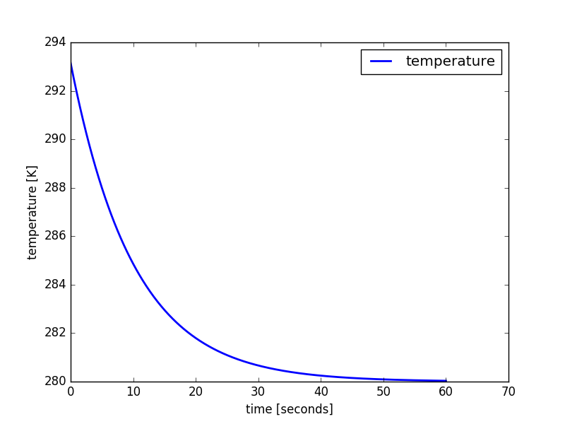
The linear decay model results
The full code can be found in the Examples section.