Examples

Linear decay equation

This is the full code from the Setting up a model section.

# import the module
import numericalmodel
from numericalmodel.interfaces import *
from numericalmodel.numericalschemes import *

# create a model
model = numericalmodel.numericalmodel.NumericalModel()
model.initial_time = 0

# define values
temperature = StateVariable( id = "T", name = "temperature", unit = "K"  )
parameter = Parameter( id = "a", name = "linear parameter", unit = "1/s"  )
forcing = ForcingValue( id = "F", name = "forcing parameter", unit = "K/s" )

# add the values to the model
model.variables  = SetOfStateVariables( [ temperature  ]  )
model.parameters = SetOfParameters(     [ parameter  ]    )
model.forcing    = SetOfForcingValues(  [ forcing  ]      )

# set initial values
model.variables["T"].value  = 20 + 273.15
model.parameters["a"].value = 0.1
model.forcing["F"].value    = 28

# define the equation
class LinearDecayEquation(numericalmodel.equations.PrognosticEquation):
    """
    Class for the linear decay equation
    """
    def linear_factor(self, time = None ):
        # take the "a" parameter from the input, interpolate it to the given
        # "time" and return the negative value
        return - self.input["a"](time)

    def independent_addend(self, time = None ):
        # take the "F" forcing parameter from the input, interpolate it to
        # the given "time" and return it
        return self.input["F"](time)

    def nonlinear_addend(self, *args, **kwargs):
        return 0 # nonlinear addend is always zero (LINEAR decay equation)

# create an equation object
decay_equation = LinearDecayEquation(
    variable = temperature,
    input = SetOfInterfaceValues( [parameter, forcing] ),
    )

# create a numerical scheme
implicit_scheme = numericalmodel.numericalschemes.EulerImplicit(
    equation = decay_equation
    )

# add the numerical scheme to the model
model.numericalschemes = SetOfNumericalSchemes( [ implicit_scheme ] )

# integrate the model
model.integrate( final_time = model.model_time + 60 )

# plot the results
import matplotlib.pyplot as plt

plt.plot( temperature.times, temperature.values,
    linewidth = 2,
    label = temperature.name,
    )
plt.xlabel( "time [seconds]" )
plt.ylabel( "{} [{}]".format( temperature.name, temperature.unit ) )
plt.legend()
plt.show()

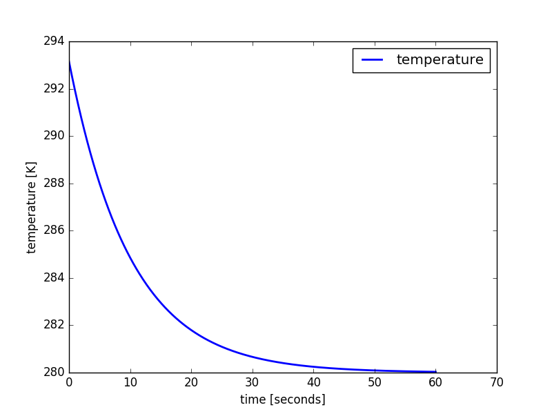
The linear decay model results

Heat transfer equation

This is an implementation of the heat transfer equation to simulate heat transfer between two reservoirs:

\[c_1 m_1 \frac{dT_1}{dt} = - a \cdot ( T_2 - T_1 )\]

\[c_2 m_2 \frac{dT_2}{dt} = - a \cdot ( T_1 - T_2 )\]

# system module
import logging

# own modules
import numericalmodel
from numericalmodel.numericalmodel import NumericalModel
from numericalmodel.interfaces import *
from numericalmodel.equations import *
from numericalmodel.numericalschemes import *

# external modules
import numpy as np
import matplotlib.pyplot as plt

logging.basicConfig(level = logging.INFO)

model = NumericalModel()
model.name = "simple heat transfer model"

### Variables ###
temperature_1 = StateVariable(id = "T1", name = "air temperature",   unit = "K")
temperature_2 = StateVariable(id = "T2", name = "water temperature", unit = "K")

### Parameters ###
transfer_parameter = Parameter(
    id = "a", name = "heat transfer parameter", unit = "W/K")
spec_heat_capacity_1 = Parameter(
    id = "c1", name = "specific heat capacity of dry air", unit = "J/(kg*K)")
spec_heat_capacity_2 = Parameter(
    id = "c2", name = "specific heat capacity of water", unit = "J/(kg*K)")
mass_1 = Parameter(id = "m1", name = "mass of air", unit = "kg")
mass_2 = Parameter(id = "m2", name = "mass of water", unit = "kg")

# add variables and parameters to model
model.variables = \
    SetOfStateVariables( [temperature_1, temperature_2] )
model.parameters = \
    SetOfParameters( [ transfer_parameter, spec_heat_capacity_1,
    spec_heat_capacity_2, mass_1, mass_2, ] )

### set initial values ###
model.initial_time = 0
temperature_1.value = 30 + 273.15
temperature_2.value = 10 + 273.15
mass_1.value = 20
mass_2.value = 10
spec_heat_capacity_1.value = 1005
spec_heat_capacity_2.value = 4190
transfer_parameter.value = 1.5

### define the heat transfer equation ###
class HeatTransferEquation( PrognosticEquation ):
    """
    Heat transfer equation:
        c1 * m1 * dT1/dt = a * ( T2 - T1 )
        c2 * m2 * dT2/dt = a * ( T1 - T2 )
    """
    def linear_factor( self, time = None ):
        v = lambda var: self.input[var](time)
        res = {
            "T1" : - v("a") / ( v("c1") * v("m1") ) ,
            "T2" : - v("a") / ( v("c2") * v("m2") ) ,
            }
        return res.get(self.variable.id,0)

    def nonlinear_addend( self, *args, **kwargs ):
        return 0

    def independent_addend( self, time = None ):
        v = lambda var: self.input[var](time)
        res = {
            "T1": v("a") * v("T2") / ( v("c1") * v("m1") ),
            "T2": v("a") * v("T1") / ( v("c2") * v("m2") ),
            }
        return res.get(self.variable.id,0)

# define equation input
equation_input = SetOfInterfaceValues( [
    temperature_1, temperature_2, transfer_parameter, spec_heat_capacity_1,
    spec_heat_capacity_2, mass_1, mass_2,
    ])

# set up equations
transfer_equation_1 = \
    HeatTransferEquation( variable = temperature_1, input = equation_input )
transfer_equation_2 = \
    HeatTransferEquation( variable = temperature_2, input = equation_input )

### numerical schemes ###
model.numericalschemes = SetOfNumericalSchemes( [
    EulerExplicit( equation = transfer_equation_1 ),
    EulerExplicit( equation = transfer_equation_2 ),
    ] )

# integrate the model
model.integrate( final_time = model.model_time + 3600 * 24 )

### calculate the analytical stationary solution ###
v = lambda var: equation_input[var].value
stationary_temperature = \
    ( v("c1") * v("m1") * v("T1") + v("c2") * v("m2") * v("T2") ) \
    / ( v("c1") * v("m1") + v("c2") * v("m2") )

logging.info("stationary solution: {}".format(stationary_temperature))
logging.info("    air temperature: {}".format(temperature_1.value))
logging.info("  water temperature: {}".format(temperature_2.value))

### Plot ###
fig, ax = plt.subplots()
ax.set_title(model.name)
ax.plot( ( temperature_1.times.min()/3600, temperature_1.times.max()/3600 ),
         ( stationary_temperature, stationary_temperature ),
         linewidth = 2,
         label = "analytical stationary solution",
         )
ax.plot( temperature_1.times/3600, temperature_1.values,
    linewidth = 2,
    label = temperature_1.name,
    )
ax.plot( temperature_2.times/3600, temperature_2.values,
    linewidth = 2,
    label = temperature_2.name,
    )
ax.set_xlabel( "time [hours]" )
ax.set_ylabel( "temperature [{}]".format( temperature_1.unit ) )
ax.legend()
plt.show()

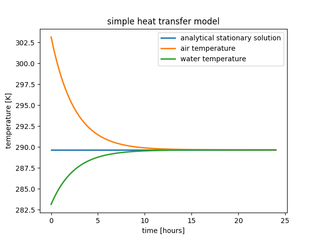
heat transfer model results